pacman::p_load(tmap, tidyverse, sf)In Class Exercise 3: Analytical Mapping
Overview
Learning Outcome
Learning how to use
Importing geospatial data in rds format into R environment.
Creating cartographic quality choropleth maps by using appropriate tmap functions.
Creating rate map
Creating percentile map
Creating boxmap
Getting Started
Installing and loading of packages
Importing of data
NGA_wp <- read_rds("data/rds/NGA_wp.rds")Basic Choropleth Mapping
Visualising distribution of non-functional water point
p1 <- tm_shape(NGA_wp) +
  tm_fill("wp_functional",
          n = 10,
          style = "equal",
          palette = "Blues") +
  tm_borders(lwd = 0.1,
             alpha = 1) +
  tm_layout(main.title = "Distribution of functional water point by LGAs",
            legend.outside = FALSE)
p2 <- tm_shape(NGA_wp) +
tm_fill("total_wp",
n = 10,
style = "equal",
palette = "Blues") +
tm_borders(lwd = 0.1,
alpha = 1) +
tm_layout(main.title = "Distribution of total water point by LGAs",
legend.outside = FALSE)tmap_arrange(p2, p1, nrow = 1)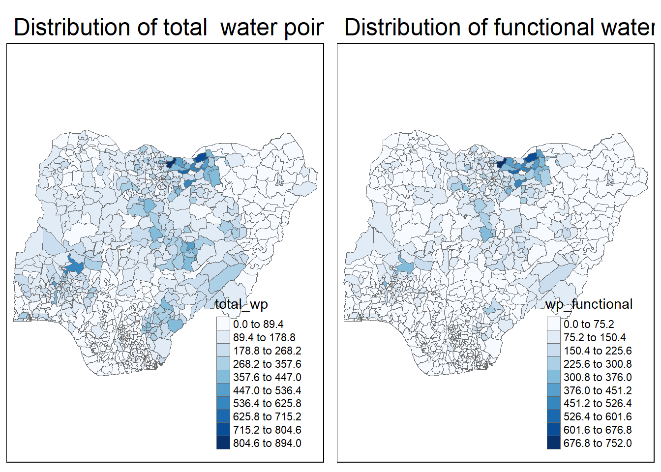
Choropleth Map for Rates
Deriving Proportion of Functional Water Points and Non-Functional Water Points
NGA_wp <- NGA_wp %>%
  mutate(pct_functional = wp_functional/total_wp) %>%
  mutate(pct_nonfunctional = wp_nonfunctional/total_wp)
Note
mutate() from dplyr package is used to derive two fields, namely pct_functional and pct_nonfunctional.
Plotting map of rate
tm_shape(NGA_wp) +
  tm_fill("pct_functional",
          n = 10,
          style = "equal",
          palette = "Blues",
          legend.hist = TRUE) +
  tm_borders(lwd = 0.1,
             alpha = 1) +
  tm_layout(main.title = "Rate map of functional water point by LGAs",
            legend.outside = TRUE)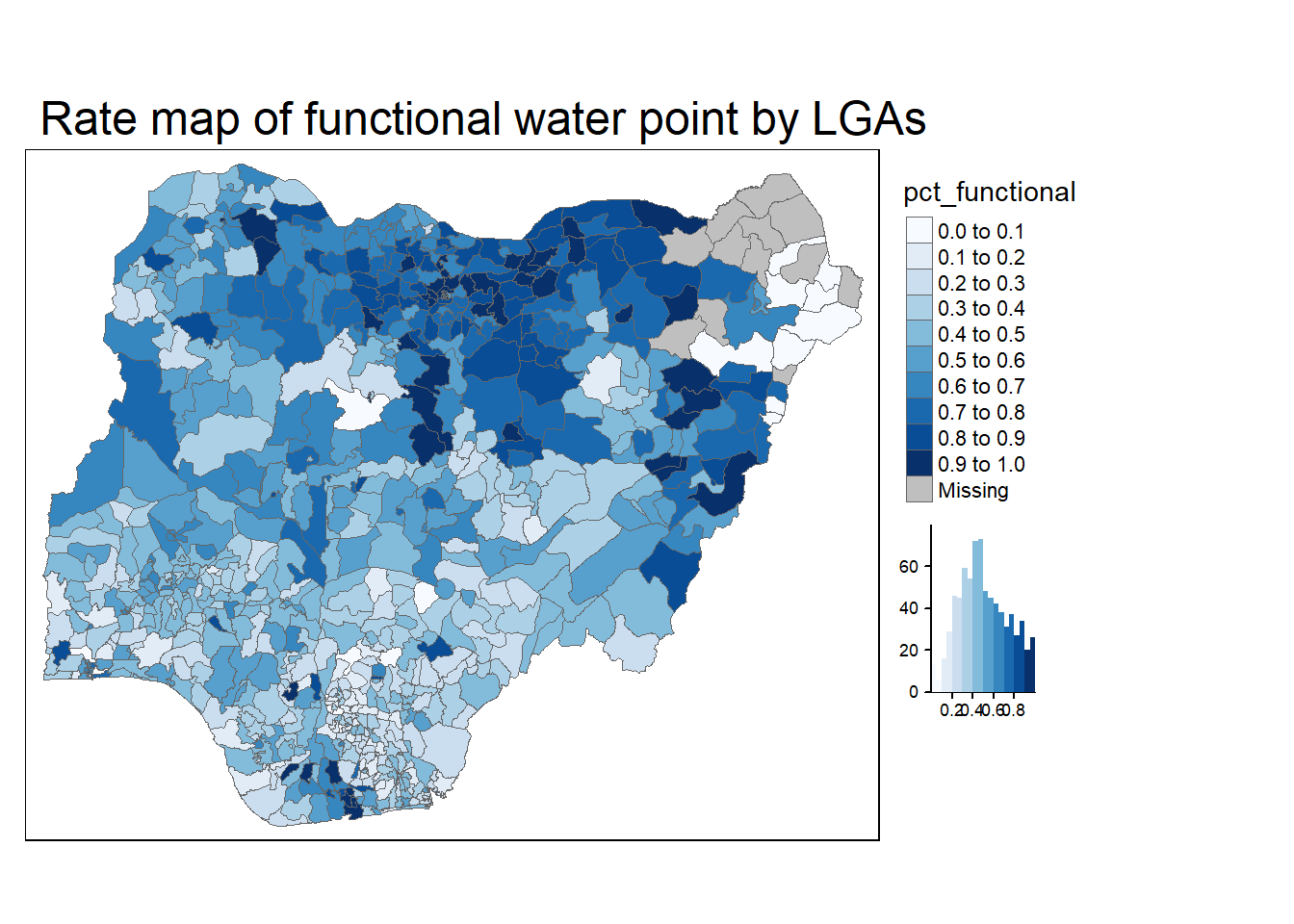
Extreme Value Maps
To highlight extreme values at lower and upper end of the scale
Percentile Map
The percentile map is a special type of quantile map with six specific categories: 0-1%,1-10%, 10-50%,50-90%,90-99%, and 99-100%.
Data Prep
Step 1: Exclude NA records
NGA_wp <- NGA_wp %>%
  drop_na()
Step 2: Creating customised classification and extracting values
percent <- c(0,.01,.1,.5,.9,.99,1)
var <- NGA_wp["pct_functional"] %>%
  st_set_geometry(NULL)
quantile(var[,1], percent)
0% 1% 10% 50% 90% 99% 100%
0.0000000 0.0000000 0.2169811 0.4791667 0.8611111 1.0000000 1.0000000
Note
When variables are extracted from an sf data.frame, the geometry is extracted as well. For mapping and spatial manipulation, this is the expected behavior, but many base R functions cannot deal with the geometry. Specifically, the quantile() gives an error. As a result st_set_geomtry(NULL) is used to drop geomtry field.
Creating get.var function
arguments:
vname: variable name (as character, in quotes)
df: name of sf data frame
returns:
- v: vector with values (without a column name)
get.var <- function(vname,df) {
  v <- df[vname] %>%
    st_set_geometry(NULL)
  v <- unname(v[,1])
  return(v)
}
A percentile mapping function
percentmap <- function(vnam, df, legtitle=NA, mtitle="Percentile Map"){
  percent <- c(0,.01,.1,.5,.9,.99,1)
  var <- get.var(vnam, df)
  bperc <- quantile(var, percent)
  tm_shape(df) +
  tm_polygons() +
  tm_shape(df) +
     tm_fill(vnam,
             title=legtitle,
             breaks=bperc,
             palette="Blues",
          labels=c("< 1%", "1% - 10%", "10% - 50%", "50% - 90%", "90% - 99%", "> 99%"))  +
  tm_borders() +
  tm_layout(main.title = mtitle,
            title.position = c("right","bottom"))
}
Test drive percentile mapping function
percentmap("total_wp", NGA_wp)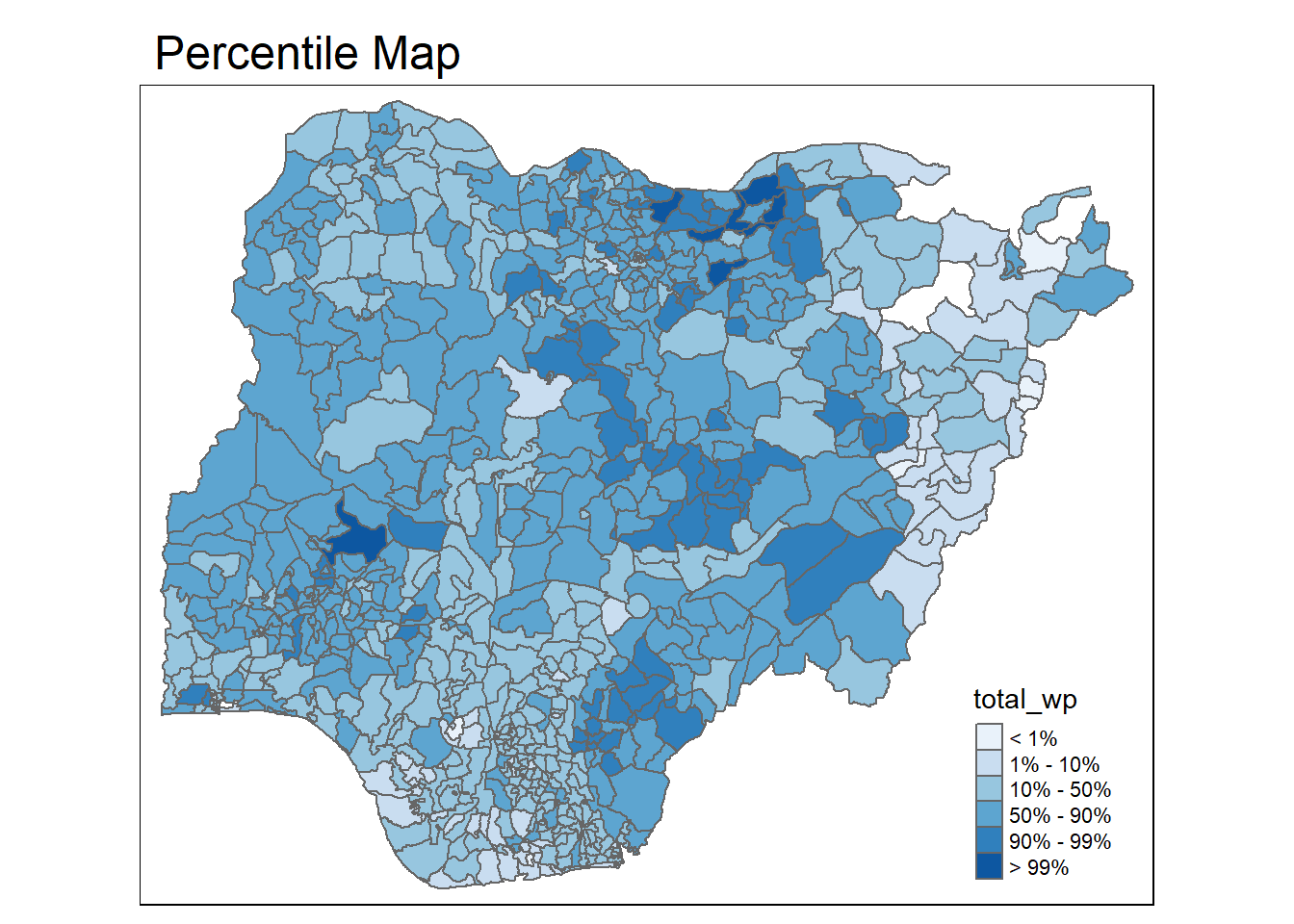
Box Map
ggplot(data = NGA_wp,
       aes(x = "",
           y = wp_nonfunctional)) +
  geom_boxplot()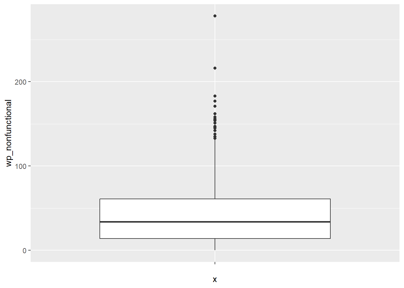
Creating boxbreaks function
arguments:
v: vector with observations
mult: multiplier for IQR (default 1.5)
returns:
- bb: vector with 7 break points compute quartile and fences
boxbreaks <- function(v,mult=1.5) {
  qv <- unname(quantile(v))
  iqr <- qv[4] - qv[2]
  upfence <- qv[4] + mult * iqr
  lofence <- qv[2] - mult * iqr
  # initialize break points vector
  bb <- vector(mode="numeric",length=7)
  # logic for lower and upper fences
  if (lofence < qv[1]) {  # no lower outliers
    bb[1] <- lofence
    bb[2] <- floor(qv[1])
  } else {
    bb[2] <- lofence
    bb[1] <- qv[1]
  }
  if (upfence > qv[5]) { # no upper outliers
    bb[7] <- upfence
    bb[6] <- ceiling(qv[5])
  } else {
    bb[6] <- upfence
    bb[7] <- qv[5]
  }
  bb[3:5] <- qv[2:4]
  return(bb)
}
Creating get.var function
arguments:
vname: variable name (as character, in quotes)
df: name of sf data frame
returns:
- v: vector with values (without a column name)
get.var <- function(vname,df) {
  v <- df[vname] %>% st_set_geometry(NULL)
  v <- unname(v[,1])
  return(v)
}
Testing created function
var <- get.var("wp_nonfunctional", NGA_wp)
boxbreaks(var)
[1] -56.5 0.0 14.0 34.0 61.0 131.5 278.0Boxmap function
boxmap <- function(vnam, df,
                   legtitle=NA,
                   mtitle="Box Map",
                   mult=1.5){
  var <- get.var(vnam,df)
  bb <- boxbreaks(var)
  tm_shape(df) +
    tm_polygons() +
  tm_shape(df) +
     tm_fill(vnam,title=legtitle,
             breaks=bb,
             palette="Blues",
          labels = c("lower outlier",
                     "< 25%",
                     "25% - 50%",
                     "50% - 75%",
                     "> 75%",
                     "upper outlier"))  +
  tm_borders() +
  tm_layout(main.title = mtitle,
            title.position = c("left",
                               "top"))
}tmap_mode("plot")
boxmap("wp_nonfunctional", NGA_wp)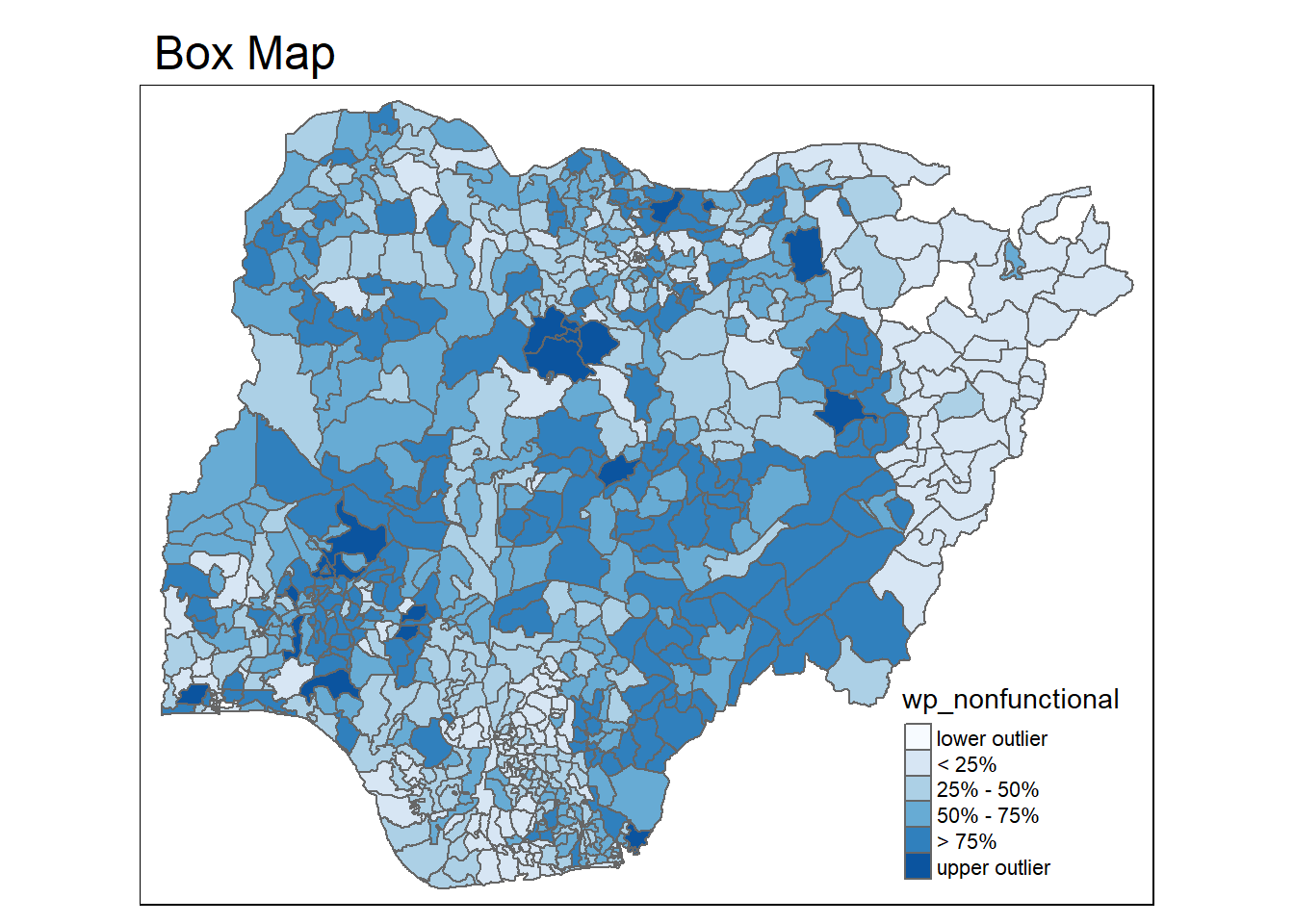
Recode Zero
Recode LGAs with zero total water point into NA.
NGA_wp <- NGA_wp %>%
  mutate(wp_functional = na_if(
    total_wp, total_wp < 0))