pacman::p_load(sf, sfdep, tmap, tidyverse, plotly)In Class Exercise 7 - GLSA
1. Installing packages
2. Importing Data
2.1 Importing Shape File
hunan <- st_read(dsn = "data/geospatial",
                 layer = "Hunan")
Reading layer `Hunan' from data source
`C:\Users\Daniel\Desktop\Github\IS419\IS415-GAA\In-Class_Ex\In-Class_Ex07\data\geospatial'
using driver `ESRI Shapefile'
Simple feature collection with 88 features and 7 fields
Geometry type: POLYGON
Dimension: XY
Bounding box: xmin: 108.7831 ymin: 24.6342 xmax: 114.2544 ymax: 30.12812
Geodetic CRS: WGS 842.2 Importing csv file
hunan2012 <- read_csv("data/aspatial/Hunan_2012.csv")2.3 Joining them together
hunan_GDPPC <- left_join(hunan,hunan2012) %>%
  select(1:4, 7, 15)
2.4 Plotting Choropleth map
tmap_mode("plot")
tm_shape(hunan_GDPPC) +
  tm_fill("GDPPC",
          style = "quantile",
          palette = "Blues",
          title = "GDPPC") +
  tm_layout(main.title = "Distribution of GDP per capita by district, Hunan Province",
            main.title.position = "center",
            main.title.size = 1.2,
            legend.height = 0.45,
            legend.width = 0.35,
            frame = TRUE) +
  tm_borders(alpha = 0.5) +
  tm_compass(type="8star", size = 2) +
  tm_scale_bar() +
  tm_grid(alpha = 0.2)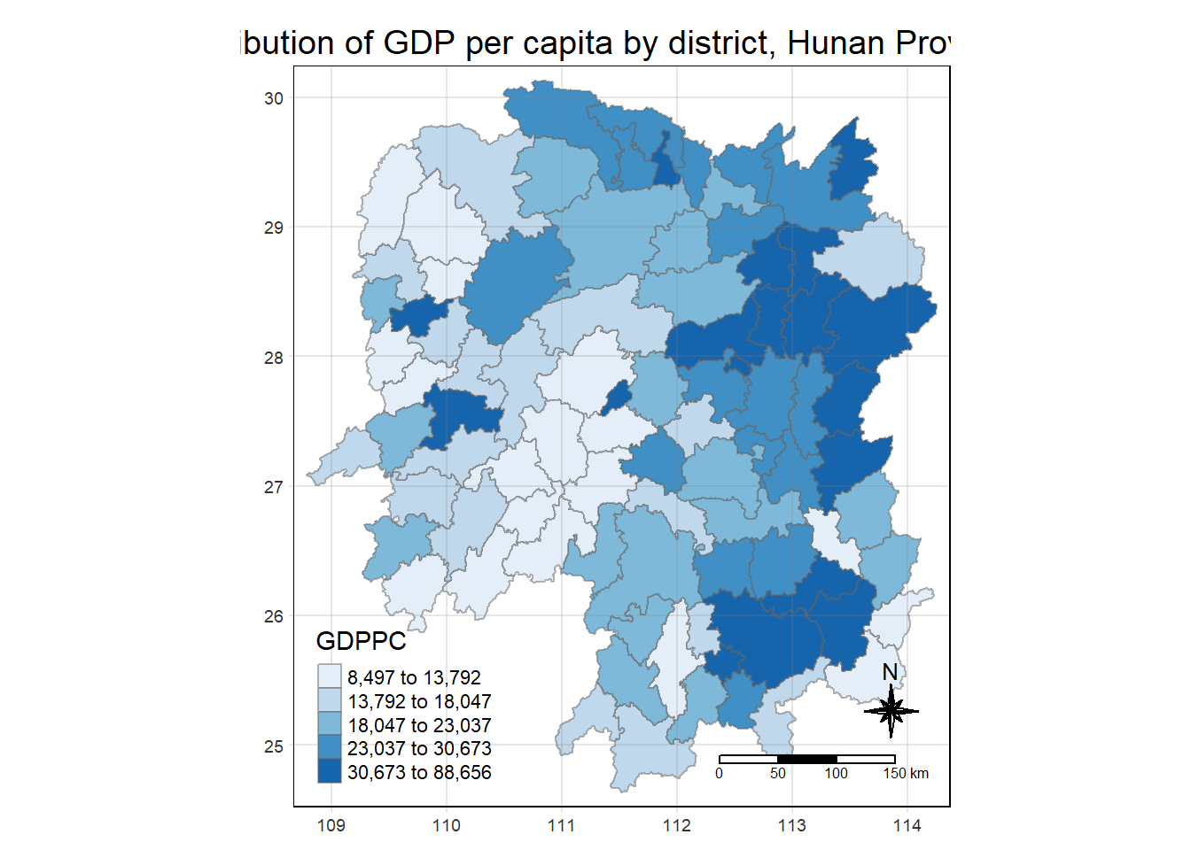
3. Global Measures of Spatial Association
3.1 Deriving contiguity weights: Queen Method
wm_q <- hunan_GDPPC %>%
  mutate(nb = st_contiguity(geometry),
         wt = st_weights(nb,
                         style = "W"),
         .before = 1)
3.2 Computing Global Moran’ I
moranI <- global_moran(wm_q$GDPPC,
                       wm_q$nb,
                       wm_q$wt)
3.3 Performing Global Moran’I Test
global_moran_test(wm_q$GDPPC,
                       wm_q$nb,
                       wm_q$wt)
    Moran I test under randomisation

data:  x
weights: listw

Moran I statistic standard deviate = 4.7351, p-value = 1.095e-06
alternative hypothesis: greater
sample estimates:
Moran I statistic       Expectation          Variance
      0.300749970      -0.011494253       0.004348351
3.4 Performing Global Moran’I Permutation Test
Note
Remember to set seed value so that the result will be consistent (Put outside to make seed standard)
set.seed(1234)global_moran_perm(wm_q$GDPPC,
wm_q$nb,
wm_q$wt,
nsim = 99)
    Monte-Carlo simulation of Moran I

data:  x
weights: listw
number of simulations + 1: 100

statistic = 0.30075, observed rank = 100, p-value < 2.2e-16
alternative hypothesis: two.sided
3.5 Computing Local Moran’s I
lisa <- wm_q %>%
  mutate(local_moran = local_moran(GDPPC, nb, wt, nsim = 99),
         .before = 1) %>%
  unnest(local_moran)
lisa
Simple feature collection with 88 features and 20 fields
Geometry type: POLYGON
Dimension: XY
Bounding box: xmin: 108.7831 ymin: 24.6342 xmax: 114.2544 ymax: 30.12812
Geodetic CRS: WGS 84
# A tibble: 88 × 21
ii eii var_ii z_ii p_ii p_ii_…¹ p_fol…² skewn…³ kurtosis
<dbl> <dbl> <dbl> <dbl> <dbl> <dbl> <dbl> <dbl> <dbl>
1 -0.00147 0.00177 4.18e-4 -0.158 0.874 0.82 0.41 -0.812 0.652
2 0.0259 0.00641 1.05e-2 0.190 0.849 0.96 0.48 -1.09 1.89
3 -0.0120 -0.0374 1.02e-1 0.0796 0.937 0.76 0.38 0.824 0.0461
4 0.00102 -0.0000349 4.37e-6 0.506 0.613 0.64 0.32 1.04 1.61
5 0.0148 -0.00340 1.65e-3 0.449 0.654 0.5 0.25 1.64 3.96
6 -0.0388 -0.00339 5.45e-3 -0.480 0.631 0.82 0.41 0.614 -0.264
7 3.37 -0.198 1.41e+0 3.00 0.00266 0.08 0.04 1.46 2.74
8 1.56 -0.265 8.04e-1 2.04 0.0417 0.08 0.04 0.459 -0.519
9 4.42 0.0450 1.79e+0 3.27 0.00108 0.02 0.01 0.746 -0.00582
10 -0.399 -0.0505 8.59e-2 -1.19 0.234 0.28 0.14 -0.685 0.134
# … with 78 more rows, 12 more variables: mean <fct>, median <fct>,
# pysal <fct>, nb <nb>, wt <list>, NAME_2 <chr>, ID_3 <int>, NAME_3 <chr>,
# ENGTYPE_3 <chr>, County <chr>, GDPPC <dbl>, geometry <POLYGON [°]>, and
# abbreviated variable names ¹p_ii_sim, ²p_folded_sim, ³skewness3.6 Visualizing local Moran’s I
tmap_mode("plot")
tm_shape(lisa) +
  tm_fill("ii") +
  tm_borders(alpha = 0.5) +
  tm_view(set.zoom.limits = c(6,8))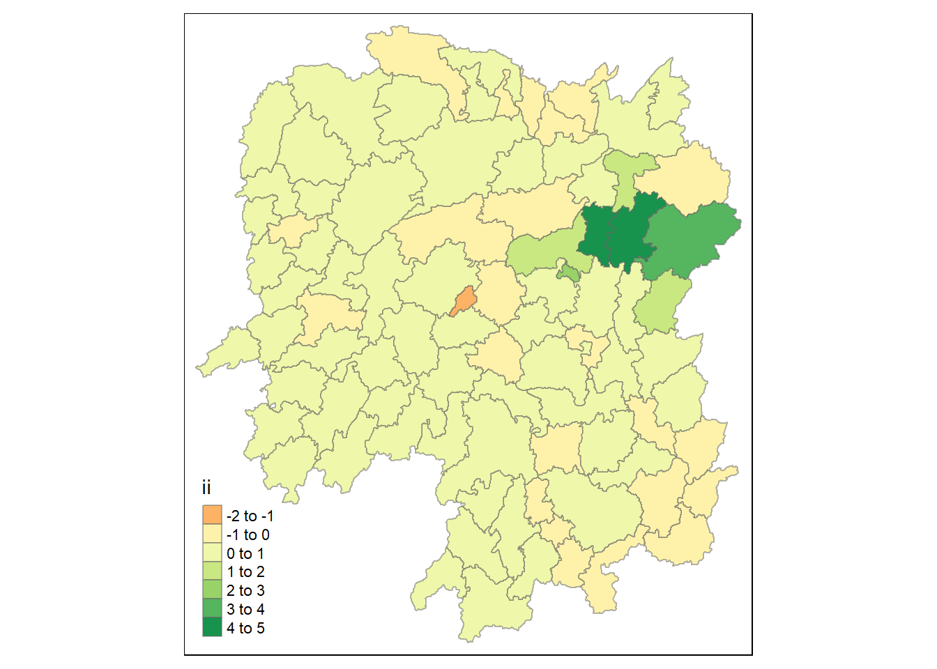
3.7 Visualizing the simulated one
tmap_mode("plot")
tm_shape(lisa) +
  tm_fill("p_ii_sim") +
  tm_borders(alpha = 0.5)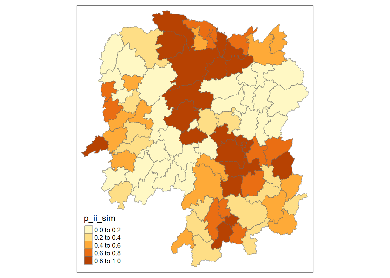
3.8 Visualizing local Moran’s I
lisa_sig <- lisa %>%
  filter(p_ii <0.05)
tmap_mode("plot")
tm_shape(lisa) +
  tm_polygons() +
  tm_borders(alpha = 0.5) +
tm_shape(lisa_sig) +
  tm_fill("mean") +
  tm_borders(alpha = 0.4)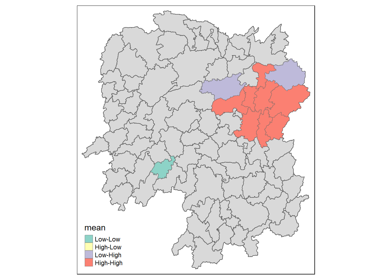
4. Hot Spot and Cold Spot Area Analysis
4.1 Computing local Moran’s I
HCSA <- wm_q %>%
  mutate(local_Gi = local_gstar_perm(
    GDPPC, nb, wt, nsim = 99),
    .before = 1) %>%
  unnest(local_Gi)
HCSA
Simple feature collection with 88 features and 16 fields
Geometry type: POLYGON
Dimension: XY
Bounding box: xmin: 108.7831 ymin: 24.6342 xmax: 114.2544 ymax: 30.12812
Geodetic CRS: WGS 84
# A tibble: 88 × 17
gi_star e_gi var_gi p_value p_sim p_fol…¹ skewn…² kurto…³ nb wt
<dbl> <dbl> <dbl> <dbl> <dbl> <dbl> <dbl> <dbl> <nb> <lis>
1 0.0416 0.0114 0.00000641 0.0493 9.61e-1 0.7 0.35 0.875 <int> <dbl>
2 -0.333 0.0106 0.00000384 -0.0941 9.25e-1 1 0.5 0.661 <int> <dbl>
3 0.281 0.0126 0.00000751 -0.151 8.80e-1 0.9 0.45 0.640 <int> <dbl>
4 0.411 0.0118 0.00000922 0.264 7.92e-1 0.6 0.3 0.853 <int> <dbl>
5 0.387 0.0115 0.00000956 0.339 7.34e-1 0.62 0.31 1.07 <int> <dbl>
6 -0.368 0.0118 0.00000591 -0.583 5.60e-1 0.72 0.36 0.594 <int> <dbl>
7 3.56 0.0151 0.00000731 2.61 9.01e-3 0.06 0.03 1.09 <int> <dbl>
8 2.52 0.0136 0.00000614 1.49 1.35e-1 0.2 0.1 1.12 <int> <dbl>
9 4.56 0.0144 0.00000584 3.53 4.17e-4 0.04 0.02 1.23 <int> <dbl>
10 1.16 0.0104 0.00000370 1.82 6.86e-2 0.12 0.06 0.416 <int> <dbl>
# … with 78 more rows, 7 more variables: NAME_2 <chr>, ID_3 <int>,
# NAME_3 <chr>, ENGTYPE_3 <chr>, County <chr>, GDPPC <dbl>,
# geometry <POLYGON [°]>, and abbreviated variable names ¹p_folded_sim,
# ²skewness, ³kurtosis4.2 Visualizing Gi*
tmap_mode("view")
tm_shape(HCSA) +
tm_fill("gi_star") +
tm_borders(alpha = 0.5) +
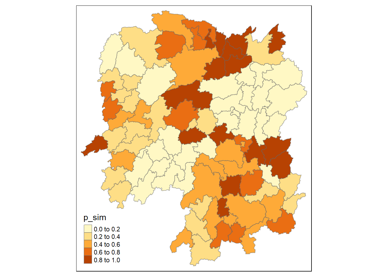
tm_view(set.zoom.limit = c(6,8))4.3 Visualizing p-value of HCSA
tmap_mode("plot")
tm_shape(HCSA) +
  tm_fill("p_sim") +
  tm_borders(alpha = 0.5)