In Class Exercise 6

Note

Note, HONs uses spdep but ICE uses sfdep

always clear environment when working on different project.

1. Getting started

1.1 Importing Packages

pacman::p_load(sf, sfdep, tmap, tidyverse)

1.2 Importing Shapefile Data

hunan <- st_read(dsn = "data/geospatial", 
                 layer = "Hunan")

Reading layer `Hunan' from data source 
  `C:\Users\Daniel\Desktop\Github\IS419\IS415-GAA\In-Class_Ex\In-Class_Ex06\data\geospatial' 
  using driver `ESRI Shapefile'
Simple feature collection with 88 features and 7 fields
Geometry type: POLYGON
Dimension:     XY
Bounding box:  xmin: 108.7831 ymin: 24.6342 xmax: 114.2544 ymax: 30.12812
Geodetic CRS:  WGS 84

1.3 Importing CSV file

hunan2012 <- read_csv("data/aspatial/Hunan_2012.csv")

1.4 Combining Both Data Frame by using left join

Note

More details on JOINS for dplyr https://statisticsglobe.com/r-dplyr-join-inner-left-right-full-semi-anti

hunan_GDPPC <- left_join(hunan,hunan2012)%>%
  select(1:4, 7, 15)

Note

Note: When joining, upper and lower case will cause problems with joining. So can specify which is the join field so prevent this from happening. For this case, we did not because its the same casing and its smart enough to detect to join by Country.

1.5 Visualising

tmap_mode("plot")
tm_shape(hunan_GDPPC) +
  tm_fill("GDPPC",
          style = "quantile",
          palette = "Blues",
          title = "GDPPC") +
  tm_layout(main.title = "Distribution of GDP per capita by distribution",
            main.title.position = "center",
            main.title.size = 0.6,
            legend.height = 0.45,
            legend.width = 0.35,
            frame = TRUE) +
  tm_borders(alpha = 0.5) +
  tm_compass(type = "8star", size = 2) +
  tm_scale_bar() + 
  tm_grid(alpha = 0.2)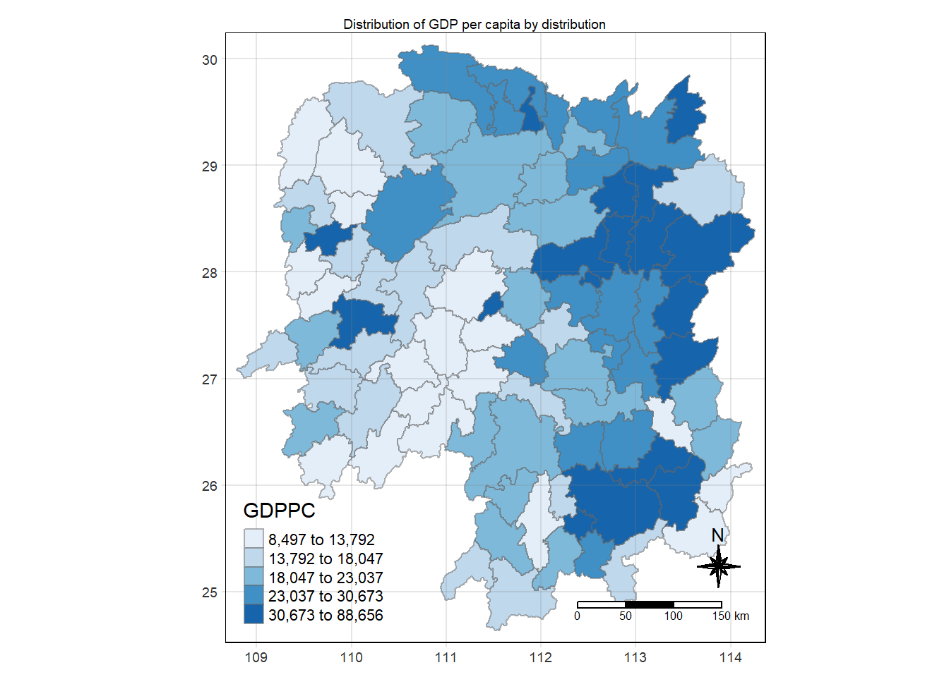

2. Contiguity Neighbor method

Note

st_contiguity() is used to derive a contiguity neighbor list by using Queen’s method

cn_queen <- hunan_GDPPC %>%
  mutate(nb = st_contiguity(geometry),
         .before = 1)

Note

Usage

st_contiguity(geometry, queen = TRUE, …)

https://sfdep.josiahparry.com/reference/st_contiguity.html

poly2nb <- this is for SP format

st_contiguity <- this is for SF format

.before <- put the newly create field in the first column

2.2 Derive contiguity neighbour list using Rook’s method

cn_rook <- hunan_GDPPC %>%
  mutate(nb = st_contiguity(geometry),
         queen = FALSE,
         .before = 1)

Note

Bishop method cant be done here. Only in spdep

3. Computing contiguity weights

3.1 Queen’s method

wm_q <- hunan_GDPPC %>%
  mutate(nb = st_contiguity(geometry),
         wt = st_weights(nb),
         .before = 1)

Note

Combine the method together

• First, generate the st_contiguity

• Then calculate the weight

So can save 1 chunk of code

3.2 Rooks method

wm_r <- hunan_GDPPC %>%
  mutate(nb = st_contiguity(geometry),
         queen = FALSE,
         wt = st_weights(nb),
         .before = 1)