packages <- c('sf', 'tidyverse', 'tmap', 'httr', 'jsonlite', 'rvest', 'sp', 'ggpubr', 'corrplot', 'broom', 'olsrr', 'spdep', 'GWmodel', 'devtools', 'rgeos', 'lwgeom', 'maptools', 'matrixStats', 'units', 'gtsummary', 'Metrics', 'rsample', 'SpatialML')
for(p in packages){
if(!require(p, character.only = T)){
install.packages(p, repos = "http://cran.us.r-project.org")
}
library(p, character.only = T)
}Take Home Exercise 3
Predicting HDB Public Housing Resale Pricies using Geographically Weighted Methods
Assignment Doc: Here
1 Setting Scene
Housing is an essential component of household wealth worldwide. Buying a housing has always been a major investment for most people. The price of housing is affected by many factors. Some of them are global in nature such as the general economy of a country or inflation rate. Others can be more specific to the properties themselves. These factors can be further divided to structural and locational factors. Structural factors are variables related to the property themselves such as the size, fitting, and tenure of the property. Locational factors are variables related to the neighbourhood of the properties such as proximity to childcare centre, public transport service and shopping centre.
Conventional, housing resale prices predictive models were built by using Ordinary Least Square (OLS) method. However, this method failed to take into consideration that spatial autocorrelation and spatial heterogeneity exist in geographic data sets such as housing transactions. With the existence of spatial autocorrelation, the OLS estimation of predictive housing resale pricing models could lead to biased, inconsistent, or inefficient results (Anselin 1998). In view of this limitation, Geographical Weighted Models were introduced for calibrating predictive model for housing resale prices.
1.1 Task
In this take-home exercise, you are tasked to predict HDB resale prices at the sub-market level (i.e. HDB 3-room, HDB 4-room and HDB 5-room) for the month of January and February 2023 in Singapore. The predictive models must be built by using by using conventional OLS method and GWR methods. You are also required to compare the performance of the conventional OLS method versus the geographical weighted methods.
1.2 Data
For the purpose of this take-home exercise, HDB Resale Flat Prices provided by Data.gov.sg should be used as the core data set. The study should focus on either three-room, four-room or five-room flat and transaction period should be from 1st January 2021 to 31st December 2022. The test data should be January and February 2023 resale prices.
Below is a list of recommended predictors to consider. However, students are free to include other appropriate independent variables.
Structural factors
Area of the unit
Floor level
Remaining lease
Age of the unit
Main Upgrading Program (MUP) completed (optional)
Locational factors
Proxomity to CBD
Proximity to eldercare
Proximity to foodcourt/hawker centres
Proximity to MRT
Proximity to park
Proximity to good primary school
Proximity to shopping mall
Proximity to supermarket
Numbers of kindergartens within 350m
Numbers of childcare centres within 350m
Numbers of bus stop within 350m
Numbers of primary school within 1km
1.3 Our Data
1.3.1 Aspatial Data
HDB Resale Data - Here
1.3.2 Geospatial Data
Master Plan 2019 Sub Zone Boundary - From Prof Kam
Shopping Malls - Referenced from Github and crossed checked with Wikipedia
MRT Stations and Bus Stops - Here
Other locations - Here
1.4 References
Senior Megan’s - Here
2 Getting Started
2.1 Importing of Packages
2.2 Importing of Aspatial Data
resale <- read_csv("data/aspatial/resale-flat-prices-based-on-registration-date-from-jan-2017-onwards.csv")Looking at the first few values of the dataset
head(resale)# A tibble: 6 × 11
month town flat_…¹ block stree…² store…³ floor…⁴ flat_…⁵ lease…⁶ remai…⁷
<chr> <chr> <chr> <chr> <chr> <chr> <dbl> <chr> <dbl> <chr>
1 2017-01 ANG MO … 2 ROOM 406 ANG MO… 10 TO … 44 Improv… 1979 61 yea…
2 2017-01 ANG MO … 3 ROOM 108 ANG MO… 01 TO … 67 New Ge… 1978 60 yea…
3 2017-01 ANG MO … 3 ROOM 602 ANG MO… 01 TO … 67 New Ge… 1980 62 yea…
4 2017-01 ANG MO … 3 ROOM 465 ANG MO… 04 TO … 68 New Ge… 1980 62 yea…
5 2017-01 ANG MO … 3 ROOM 601 ANG MO… 01 TO … 67 New Ge… 1980 62 yea…
6 2017-01 ANG MO … 3 ROOM 150 ANG MO… 01 TO … 68 New Ge… 1981 63 yea…
# … with 1 more variable: resale_price <dbl>, and abbreviated variable names
# ¹flat_type, ²street_name, ³storey_range, ⁴floor_area_sqm, ⁵flat_model,
# ⁶lease_commence_date, ⁷remaining_lease2.2.1 Filtering Resale Data
Filtering Resales data to only include data of 4 room and months between Jan 2021 and Feb 2023
resale_filtered <- filter(resale, flat_type == "4 ROOM") %>%
filter(month >= "2021-01" & month <= "2023-02")Double Checking the Time Period
unique(resale_filtered$month) [1] "2021-01" "2021-02" "2021-03" "2021-04" "2021-05" "2021-06" "2021-07"
[8] "2021-08" "2021-09" "2021-10" "2021-11" "2021-12" "2022-01" "2022-02"
[15] "2022-03" "2022-04" "2022-05" "2022-06" "2022-07" "2022-08" "2022-09"
[22] "2022-10" "2022-11" "2022-12" "2023-01" "2023-02"Double Checking Flat Type
unique(resale_filtered$flat_type)[1] "4 ROOM"Taking a look at the filtered results
glimpse(resale_filtered)Rows: 25,502
Columns: 11
$ month <chr> "2021-01", "2021-01", "2021-01", "2021-01", "2021-…
$ town <chr> "ANG MO KIO", "ANG MO KIO", "ANG MO KIO", "ANG MO …
$ flat_type <chr> "4 ROOM", "4 ROOM", "4 ROOM", "4 ROOM", "4 ROOM", …
$ block <chr> "547", "414", "509", "467", "571", "134", "204", "…
$ street_name <chr> "ANG MO KIO AVE 10", "ANG MO KIO AVE 10", "ANG MO …
$ storey_range <chr> "04 TO 06", "01 TO 03", "01 TO 03", "07 TO 09", "0…
$ floor_area_sqm <dbl> 92, 92, 91, 92, 92, 98, 92, 92, 92, 92, 92, 109, 9…
$ flat_model <chr> "New Generation", "New Generation", "New Generatio…
$ lease_commence_date <dbl> 1981, 1979, 1980, 1979, 1979, 1978, 1977, 1978, 19…
$ remaining_lease <chr> "59 years", "57 years 09 months", "58 years 06 mon…
$ resale_price <dbl> 370000, 375000, 380000, 385000, 410000, 410000, 41…2.2.2 Adding More Data to Resale Data
2.2.2.1 Adding New Data to Dataset
Address
Remaining Lease year and months
resale_transformed <- resale_filtered %>%
mutate(resale_filtered, address = paste(block,street_name)) %>%
mutate(resale_filtered, remaining_lease_yr = as.integer(str_sub(remaining_lease, 0, 2))) %>%
mutate(resale_filtered, remaining_lease_mth = as.integer(str_sub(remaining_lease, 9, 11)))Replacing NA values to 0
resale_transformed$remaining_lease_mth[is.na(resale_transformed$remaining_lease_mth)] <- 0Converting lease years to months for easier calculation later
resale_transformed$remaining_lease_yr <- resale_transformed$remaining_lease_yr * 12
resale_transformed <- resale_transformed %>%
mutate(resale_transformed, remaining_lease_mths = rowSums(resale_transformed[, c("remaining_lease_yr", "remaining_lease_mth")])) %>%
select(month, town, address, block, street_name, flat_type, storey_range, floor_area_sqm, flat_model, lease_commence_date, remaining_lease_mths, resale_price)2.2.2.2 Getting of LAT & LONG from OneMap.sg API
For us to visualize the data on the map, we will have to first get the LAT & LONG data from the address. Its a good thing that OneMap.sg has an API for us to easily grab the LAT & LONG based off the address.
More details on how to use OneMap.sg API here
First we create a variable of all unique address
address <- sort(unique(resale_transformed$address))Viewing the first few addresses
head(address)[1] "1 CHAI CHEE RD" "1 PINE CL" "1 ST. GEORGE'S RD"
[4] "1 TECK WHYE AVE" "1 TOH YI DR" "10 CHAI CHEE RD" We will then use a function to loop through and retrieve the LAT and LONG
get_coords <- function(add_list){
# Create a data frame to store all retrieved coordinates
postal_coords <- data.frame()
for (i in add_list){
#print(i)
r <- GET('https://developers.onemap.sg/commonapi/search?',
query=list(searchVal=i,
returnGeom='Y',
getAddrDetails='Y'))
data <- fromJSON(rawToChar(r$content))
found <- data$found
res <- data$results
# Create a new data frame for each address
new_row <- data.frame()
# If single result, append
if (found == 1){
postal <- res$POSTAL
lat <- res$LATITUDE
lng <- res$LONGITUDE
new_row <- data.frame(address= i, postal = postal, latitude = lat, longitude = lng)
}
# If multiple results, drop NIL and append top 1
else if (found > 1){
# Remove those with NIL as postal
res_sub <- res[res$POSTAL != "NIL", ]
# Set as NA first if no Postal
if (nrow(res_sub) == 0) {
new_row <- data.frame(address= i, postal = NA, latitude = NA, longitude = NA)
}
else{
top1 <- head(res_sub, n = 1)
postal <- top1$POSTAL
lat <- top1$LATITUDE
lng <- top1$LONGITUDE
new_row <- data.frame(address= i, postal = postal, latitude = lat, longitude = lng)
}
}
else {
new_row <- data.frame(address= i, postal = NA, latitude = NA, longitude = NA)
}
# Add the row
postal_coords <- rbind(postal_coords, new_row)
}
return(postal_coords)
}Running the Function
latlong <- get_coords(address)Checking if there is any missing values
latlong[(is.na(latlong))]character(0)2.2.2.3 Combining the Data back
resale_latlong <- left_join(resale_transformed, latlong, by = c('address' = 'address'))Viewing the results
head(resale_latlong)# A tibble: 6 × 15
month town address block stree…¹ flat_…² store…³ floor…⁴ flat_…⁵ lease…⁶
<chr> <chr> <chr> <chr> <chr> <chr> <chr> <dbl> <chr> <dbl>
1 2021-01 ANG MO … 547 AN… 547 ANG MO… 4 ROOM 04 TO … 92 New Ge… 1981
2 2021-01 ANG MO … 414 AN… 414 ANG MO… 4 ROOM 01 TO … 92 New Ge… 1979
3 2021-01 ANG MO … 509 AN… 509 ANG MO… 4 ROOM 01 TO … 91 New Ge… 1980
4 2021-01 ANG MO … 467 AN… 467 ANG MO… 4 ROOM 07 TO … 92 New Ge… 1979
5 2021-01 ANG MO … 571 AN… 571 ANG MO… 4 ROOM 07 TO … 92 New Ge… 1979
6 2021-01 ANG MO … 134 AN… 134 ANG MO… 4 ROOM 07 TO … 98 New Ge… 1978
# … with 5 more variables: remaining_lease_mths <dbl>, resale_price <dbl>,
# postal <chr>, latitude <chr>, longitude <chr>, and abbreviated variable
# names ¹street_name, ²flat_type, ³storey_range, ⁴floor_area_sqm,
# ⁵flat_model, ⁶lease_commence_dateChecking if there is any missing values
resale_latlong[(is.na(resale_latlong))]<unspecified> [0]2.2.2.4 Saving the result into a file
Running this allows us to save the file for us to save time and from re-running the steps to retrieve the same resale file with LAT and LONG values.
resale_latlong.rds <- write_rds(resale_latlong, "data/model/resale_latlong.rds")2.2.3 Reading of Resale file with LAT and LONG
Start from this step if you already have your own resale file with the LAT and LONG data.
Remember to either change the file name to match the code or code to match the file.
resale_main <- read_rds("data/model/resale_latlong.rds")Previewing the content
head(resale_main)# A tibble: 6 × 15
month town address block stree…¹ flat_…² store…³ floor…⁴ flat_…⁵ lease…⁶
<chr> <chr> <chr> <chr> <chr> <chr> <chr> <dbl> <chr> <dbl>
1 2021-01 ANG MO … 547 AN… 547 ANG MO… 4 ROOM 04 TO … 92 New Ge… 1981
2 2021-01 ANG MO … 414 AN… 414 ANG MO… 4 ROOM 01 TO … 92 New Ge… 1979
3 2021-01 ANG MO … 509 AN… 509 ANG MO… 4 ROOM 01 TO … 91 New Ge… 1980
4 2021-01 ANG MO … 467 AN… 467 ANG MO… 4 ROOM 07 TO … 92 New Ge… 1979
5 2021-01 ANG MO … 571 AN… 571 ANG MO… 4 ROOM 07 TO … 92 New Ge… 1979
6 2021-01 ANG MO … 134 AN… 134 ANG MO… 4 ROOM 07 TO … 98 New Ge… 1978
# … with 5 more variables: remaining_lease_mths <dbl>, resale_price <dbl>,
# postal <chr>, latitude <chr>, longitude <chr>, and abbreviated variable
# names ¹street_name, ²flat_type, ³storey_range, ⁴floor_area_sqm,
# ⁵flat_model, ⁶lease_commence_date2.2.4 Transforming to sf and assigning CRS
resale_main_sf <- st_as_sf(resale_main,
coords = c("longitude", "latitude"),
crs=4326) %>%
st_transform(crs = 3414)Let’s check if the coordinate value is correct
st_crs(resale_main_sf)Coordinate Reference System:
User input: EPSG:3414
wkt:
PROJCRS["SVY21 / Singapore TM",
BASEGEOGCRS["SVY21",
DATUM["SVY21",
ELLIPSOID["WGS 84",6378137,298.257223563,
LENGTHUNIT["metre",1]]],
PRIMEM["Greenwich",0,
ANGLEUNIT["degree",0.0174532925199433]],
ID["EPSG",4757]],
CONVERSION["Singapore Transverse Mercator",
METHOD["Transverse Mercator",
ID["EPSG",9807]],
PARAMETER["Latitude of natural origin",1.36666666666667,
ANGLEUNIT["degree",0.0174532925199433],
ID["EPSG",8801]],
PARAMETER["Longitude of natural origin",103.833333333333,
ANGLEUNIT["degree",0.0174532925199433],
ID["EPSG",8802]],
PARAMETER["Scale factor at natural origin",1,
SCALEUNIT["unity",1],
ID["EPSG",8805]],
PARAMETER["False easting",28001.642,
LENGTHUNIT["metre",1],
ID["EPSG",8806]],
PARAMETER["False northing",38744.572,
LENGTHUNIT["metre",1],
ID["EPSG",8807]]],
CS[Cartesian,2],
AXIS["northing (N)",north,
ORDER[1],
LENGTHUNIT["metre",1]],
AXIS["easting (E)",east,
ORDER[2],
LENGTHUNIT["metre",1]],
USAGE[
SCOPE["Cadastre, engineering survey, topographic mapping."],
AREA["Singapore - onshore and offshore."],
BBOX[1.13,103.59,1.47,104.07]],
ID["EPSG",3414]]Lastly, we will check if there is any invalid Geometries
length(which(st_is_valid(resale_main_sf) == FALSE))[1] 02.3 Importing Geospatial Data
mpsz <- st_read(dsn = "data/geospatial", layer = "MPSZ-2019")Reading layer `MPSZ-2019' from data source
`C:\Users\Daniel\Desktop\Github\IS419\IS415-GAA\Take-Home_Ex\Take-Home_Ex03\data\geospatial'
using driver `ESRI Shapefile'
Simple feature collection with 332 features and 6 fields
Geometry type: MULTIPOLYGON
Dimension: XY
Bounding box: xmin: 103.6057 ymin: 1.158699 xmax: 104.0885 ymax: 1.470775
Geodetic CRS: WGS 84Checking if there is any invalid Geometries
length(which(st_is_valid(mpsz) == FALSE))[1] 6Since there is invalid Geometries, we will make it valid
Holes in polygons are okay, but they can cause problems if they go the wrong way round or if the hole is caused by the polygon looping itself.
mpsz <- st_make_valid(mpsz)
length(which(st_is_valid(mpsz) == FALSE))[1] 0Lastly, like the previous resale LATLONG data, we will change the CRS code
mpsz <- st_transform(mpsz, 3414)
st_crs(mpsz)Coordinate Reference System:
User input: EPSG:3414
wkt:
PROJCRS["SVY21 / Singapore TM",
BASEGEOGCRS["SVY21",
DATUM["SVY21",
ELLIPSOID["WGS 84",6378137,298.257223563,
LENGTHUNIT["metre",1]]],
PRIMEM["Greenwich",0,
ANGLEUNIT["degree",0.0174532925199433]],
ID["EPSG",4757]],
CONVERSION["Singapore Transverse Mercator",
METHOD["Transverse Mercator",
ID["EPSG",9807]],
PARAMETER["Latitude of natural origin",1.36666666666667,
ANGLEUNIT["degree",0.0174532925199433],
ID["EPSG",8801]],
PARAMETER["Longitude of natural origin",103.833333333333,
ANGLEUNIT["degree",0.0174532925199433],
ID["EPSG",8802]],
PARAMETER["Scale factor at natural origin",1,
SCALEUNIT["unity",1],
ID["EPSG",8805]],
PARAMETER["False easting",28001.642,
LENGTHUNIT["metre",1],
ID["EPSG",8806]],
PARAMETER["False northing",38744.572,
LENGTHUNIT["metre",1],
ID["EPSG",8807]]],
CS[Cartesian,2],
AXIS["northing (N)",north,
ORDER[1],
LENGTHUNIT["metre",1]],
AXIS["easting (E)",east,
ORDER[2],
LENGTHUNIT["metre",1]],
USAGE[
SCOPE["Cadastre, engineering survey, topographic mapping."],
AREA["Singapore - onshore and offshore."],
BBOX[1.13,103.59,1.47,104.07]],
ID["EPSG",3414]]2.3.1 Import Geospatial Data without LATLONG in data
CBD Area
For CBD data, we can easily find the location of CBD area according to here
From the LATLONG of 1°17′30″N 103°51′00″E according to the Wiki source, we can get the number coordinates from Google Map by placing the coordinate above, then right-clicking on the pin to get the values of 1.291667, 103.850000. It seems like the location pointed to is 3 Coleman St, Singapore 179804.
name <- c('CBD')
latitude = c(1.291667)
longitude = c(103.850000)
cbd <- data.frame(name, latitude, longitude)As usual, we will need to change the CRS value to match.
cbd_sf <- st_as_sf(cbd,
coords = c("longitude",
"latitude"),
crs = 4326) %>%
st_transform(crs = 3414)
st_crs(cbd_sf)Coordinate Reference System:
User input: EPSG:3414
wkt:
PROJCRS["SVY21 / Singapore TM",
BASEGEOGCRS["SVY21",
DATUM["SVY21",
ELLIPSOID["WGS 84",6378137,298.257223563,
LENGTHUNIT["metre",1]]],
PRIMEM["Greenwich",0,
ANGLEUNIT["degree",0.0174532925199433]],
ID["EPSG",4757]],
CONVERSION["Singapore Transverse Mercator",
METHOD["Transverse Mercator",
ID["EPSG",9807]],
PARAMETER["Latitude of natural origin",1.36666666666667,
ANGLEUNIT["degree",0.0174532925199433],
ID["EPSG",8801]],
PARAMETER["Longitude of natural origin",103.833333333333,
ANGLEUNIT["degree",0.0174532925199433],
ID["EPSG",8802]],
PARAMETER["Scale factor at natural origin",1,
SCALEUNIT["unity",1],
ID["EPSG",8805]],
PARAMETER["False easting",28001.642,
LENGTHUNIT["metre",1],
ID["EPSG",8806]],
PARAMETER["False northing",38744.572,
LENGTHUNIT["metre",1],
ID["EPSG",8807]]],
CS[Cartesian,2],
AXIS["northing (N)",north,
ORDER[1],
LENGTHUNIT["metre",1]],
AXIS["easting (E)",east,
ORDER[2],
LENGTHUNIT["metre",1]],
USAGE[
SCOPE["Cadastre, engineering survey, topographic mapping."],
AREA["Singapore - onshore and offshore."],
BBOX[1.13,103.59,1.47,104.07]],
ID["EPSG",3414]]Primary Schools
As the data given for the primary schools do not have LATLONG details, we will need to use the function created above to give us the LATLONG values again.
primary_raw <- read.csv("data/geospatial/general-information-of-schools.csv")
primary_data <- primary_raw %>%
filter(mainlevel_code == "PRIMARY") %>%
select(school_name, address, postal_code, mainlevel_code)
glimpse(primary_data)Rows: 183
Columns: 4
$ school_name <chr> "ADMIRALTY PRIMARY SCHOOL", "AHMAD IBRAHIM PRIMARY SCHO…
$ address <chr> "11 WOODLANDS CIRCLE", "10 YISHUN STREET 11", "100 …
$ postal_code <int> 738907, 768643, 579646, 159016, 544969, 569785, 569920,…
$ mainlevel_code <chr> "PRIMARY", "PRIMARY", "PRIMARY", "PRIMARY", "PRIMARY", …Calling the LATLONG conversion steps and function similar to above
primary_postal <- unique(primary_data$postal_code)
primary_latlong <- get_coords(primary_postal)Checking for NAs
primary_latlong[(is.na(primary_latlong))][1] NA NA NA NA NA NA NA NA NAAfter looking at the issue, we can see that the issue is due to postal that starts with 0, thus we will remove the 0
primary_data$postal_code[primary_data$postal_code == '88256'] <- '088256'
primary_data$postal_code[primary_data$postal_code == '99757'] <- '099757'
primary_data$postal_code[primary_data$postal_code == '99840'] <- '099840'Re-running the functions
primary_postal <- unique(primary_data$postal_code)
primary_latlong <- get_coords(primary_postal)
primary_latlong[(is.na(primary_latlong))]character(0)Now we will combine the data and convert the CRS value
primary_school <- left_join(primary_data, primary_latlong, by = c('postal_code' = 'postal'))
primary_school_sf <- st_as_sf(primary_school,
coords = c("longitude",
"latitude"),
crs = 4326) %>%
st_transform(crs = 3414)Good Primary Schools
To define good primary schools, we get the data from here. However your preferences and sources might vary, so do change as you wish
good_primary_school <- primary_school %>%
filter(school_name %in%
c("PEI HWA PRESBYTERIAN PRIMARY SCHOOL",
"GONGSHANG PRIMARY SCHOOL",
"RIVERSIDE PRIMARY SCHOOL",
"RED SWASTIKA SCHOOL",
"PUNGGOL GREEN PRIMARY SCHOOL",
"PRINCESS ELIZABETH PRIMARY SCHOOL",
"WESTWOOD PRIMARY SCHOOL",
"AI TONG SCHOOL",
"FRONTIER PRIMARY SCHOOL",
"OASIS PRIMARY SCHOOL"))As usual, converting CRS value
good_primary_school_sf <- st_as_sf(good_primary_school,
coords = c("longitude",
"latitude"),
crs = 4326) %>%
st_transform(crs = 3414)Shopping Malls
As there is source of shopping mall data from gov.sg, the source was taken from Wiki and from a person who created a scrapper to get the data with LATLONG.
shopping <- read.csv("data/geospatial/mall_coordinates.csv")
shopping <- shopping %>%
select(name, latitude, longitude)
glimpse(shopping)Rows: 199
Columns: 3
$ name <chr> "100 AM", "i12 Katong", "313@SOMERSET", "321 CLEMENTI", "600…
$ latitude <dbl> 1.274588, 1.305087, 1.301385, 1.312025, 1.334042, 1.437131, …
$ longitude <dbl> 103.8435, 103.9051, 103.8377, 103.7650, 103.8510, 103.7953, …Converting CRS
shopping_sf <- st_as_sf(shopping,
coords = c("longitude",
"latitude"),
crs = 4326) %>%
st_transform(crs = 3414)2.3.2 Importing Geospatial Data with LATLONG in data
Since all the other data sets already have LATLONG included, we will import them and ensure the CRS code is correct
Elderly Care
elder_sf <- st_read(dsn = "data/geospatial", layer = "ELDERCARE")Reading layer `ELDERCARE' from data source
`C:\Users\Daniel\Desktop\Github\IS419\IS415-GAA\Take-Home_Ex\Take-Home_Ex03\data\geospatial'
using driver `ESRI Shapefile'
Simple feature collection with 133 features and 18 fields
Geometry type: POINT
Dimension: XY
Bounding box: xmin: 14481.92 ymin: 28218.43 xmax: 41665.14 ymax: 46804.9
Projected CRS: SVY21elder_sf <- st_transform(elder_sf, 3414)Hawker Centre
hawker_sf <- st_read(dsn = "data/geospatial", layer = "HAWKERCENTRE")Reading layer `HAWKERCENTRE' from data source
`C:\Users\Daniel\Desktop\Github\IS419\IS415-GAA\Take-Home_Ex\Take-Home_Ex03\data\geospatial'
using driver `ESRI Shapefile'
Simple feature collection with 125 features and 21 fields
Geometry type: POINT
Dimension: XY
Bounding box: xmin: 12874.19 ymin: 28355.97 xmax: 45241.4 ymax: 47872.53
Projected CRS: SVY21hawker_sf <- st_transform(hawker_sf, 3414)MRT Stations
mrt <- read.csv("data/geospatial/mrtsg.csv")
mrt_sf <- st_as_sf(mrt,
coords = c("Longitude",
"Latitude"),
crs = 4326) %>%
st_transform(crs = 3414)Parks
parks_sf <- st_read(dsn = "data/geospatial", layer = "NATIONALPARKS")Reading layer `NATIONALPARKS' from data source
`C:\Users\Daniel\Desktop\Github\IS419\IS415-GAA\Take-Home_Ex\Take-Home_Ex03\data\geospatial'
using driver `ESRI Shapefile'
Simple feature collection with 352 features and 15 fields
Geometry type: POINT
Dimension: XY
Bounding box: xmin: 12373.11 ymin: 21869.93 xmax: 46735.95 ymax: 49231.09
Projected CRS: SVY21parks_sf <- st_transform(parks_sf, 3414)Supermarkets
supermarket_sf <- st_read(dsn = "data/geospatial", layer = "SUPERMARKETS")Reading layer `SUPERMARKETS' from data source
`C:\Users\Daniel\Desktop\Github\IS419\IS415-GAA\Take-Home_Ex\Take-Home_Ex03\data\geospatial'
using driver `ESRI Shapefile'
Simple feature collection with 526 features and 8 fields
Geometry type: POINT
Dimension: XY
Bounding box: xmin: 4901.188 ymin: 25529.08 xmax: 46948.22 ymax: 49233.6
Projected CRS: SVY21supermarket_sf <- st_transform(supermarket_sf, 3414)Kindergartens
kindergarten_sf <- st_read(dsn = "data/geospatial", layer = "KINDERGARTENS")Reading layer `KINDERGARTENS' from data source
`C:\Users\Daniel\Desktop\Github\IS419\IS415-GAA\Take-Home_Ex\Take-Home_Ex03\data\geospatial'
using driver `ESRI Shapefile'
Simple feature collection with 448 features and 15 fields
Geometry type: POINT
Dimension: XY
Bounding box: xmin: 11909.7 ymin: 25596.33 xmax: 43395.47 ymax: 48562.06
Projected CRS: SVY21kindergarten_sf <- st_transform(kindergarten_sf, 3414)Childcare
childcare_sf <- st_read(dsn = "data/geospatial", layer = "CHILDCARE")Reading layer `CHILDCARE' from data source
`C:\Users\Daniel\Desktop\Github\IS419\IS415-GAA\Take-Home_Ex\Take-Home_Ex03\data\geospatial'
using driver `ESRI Shapefile'
Simple feature collection with 1545 features and 15 fields
Geometry type: POINT
Dimension: XY
Bounding box: xmin: 11203.01 ymin: 25667.6 xmax: 45404.24 ymax: 49300.88
Projected CRS: WGS_1984_Transverse_Mercator# Assign EPSG Code
childcare_sf <- st_transform(childcare_sf, 3414)Bus Stops
BusStop_sf <- st_read(dsn = "data/geospatial", layer = "BusStop")Reading layer `BusStop' from data source
`C:\Users\Daniel\Desktop\Github\IS419\IS415-GAA\Take-Home_Ex\Take-Home_Ex03\data\geospatial'
using driver `ESRI Shapefile'
Simple feature collection with 5159 features and 3 fields
Geometry type: POINT
Dimension: XY
Bounding box: xmin: 3970.122 ymin: 26482.1 xmax: 48284.56 ymax: 52983.82
Projected CRS: SVY21BusStop_sf <- st_transform(BusStop_sf, 3414)3 Proximity Calculation
3.1 Function for calculation
3.1.1 Normal Calculation
Currently, the distance is measured in metre because SVY21 projected coordinate system is used. The code chunk below will be used to convert the unit f measurement from metre to km.
prox_cal <- function(df1, df2, col_name) {
dist_matrix <- st_distance(df1, df2)
df1[,col_name] <- rowMins(dist_matrix) / 1000
return(df1)
}3.1.2 With Radius Calculation
prox_cal_radius <- function(df1, df2, col_name, radius) {
dist_matrix <- st_distance(df1, df2) %>%
drop_units() %>%
as.data.frame()
df1[,col_name] <- rowSums(dist_matrix <= radius)
return(df1)
}3.2 Calculating Location Factors
Normal
resale_main_sf <- prox_cal(resale_main_sf, cbd_sf, "PROX_CBD")
resale_main_sf <- prox_cal(resale_main_sf, elder_sf, "PROX_ELDERCARE")
resale_main_sf <- prox_cal(resale_main_sf, hawker_sf, "PROX_HAWKER")
resale_main_sf <- prox_cal(resale_main_sf, mrt_sf, "PROX_MRT")
resale_main_sf <- prox_cal(resale_main_sf, parks_sf, "PROX_PARK")
resale_main_sf <- prox_cal(resale_main_sf, good_primary_school_sf, "PROX_GOODPRIMARY")
resale_main_sf <- prox_cal(resale_main_sf, shopping_sf, "PROX_SHOPPING")
resale_main_sf <- prox_cal(resale_main_sf, BusStop_sf, "PROX_BUS")
resale_main_sf <- prox_cal(resale_main_sf, childcare_sf, "PROX_CHILDCARE")
resale_main_sf <- prox_cal(resale_main_sf, supermarket_sf, "PROX_SUPERMARKET")Radius
resale_main_sf <- prox_cal_radius(resale_main_sf, kindergarten_sf, "WITHIN_350M_KINDERGARTEN", 350)
resale_main_sf <- prox_cal_radius(resale_main_sf, childcare_sf, "WITHIN_350M_CHILDCARE", 350)
resale_main_sf <- prox_cal_radius(resale_main_sf, BusStop_sf, "WITHIN_350M_BUS", 350)
resale_main_sf <- prox_cal_radius(resale_main_sf, primary_school_sf, "WITHIN_1KM_PRIMARY", 1000)3.3 Saving of dataset
resale_main_sf <- resale_main_sf %>%
mutate() %>%
rename("AREA_SQM" = "floor_area_sqm",
"LEASE_MTHS" = "remaining_lease_mths",
"PRICE" = "resale_price",
"STOREY" = "storey_range")4 EDA
resale_main_sf <- read_rds("data/model/resale_main.rds")glimpse(resale_main_sf)Rows: 25,502
Columns: 28
$ month <chr> "2021-01", "2021-01", "2021-01", "2021-01", "…
$ town <chr> "ANG MO KIO", "ANG MO KIO", "ANG MO KIO", "AN…
$ address <chr> "547 ANG MO KIO AVE 10", "414 ANG MO KIO AVE …
$ block <chr> "547", "414", "509", "467", "571", "134", "20…
$ street_name <chr> "ANG MO KIO AVE 10", "ANG MO KIO AVE 10", "AN…
$ flat_type <chr> "4 ROOM", "4 ROOM", "4 ROOM", "4 ROOM", "4 RO…
$ STOREY <chr> "04 TO 06", "01 TO 03", "01 TO 03", "07 TO 09…
$ AREA_SQM <dbl> 92, 92, 91, 92, 92, 98, 92, 92, 92, 92, 92, 1…
$ flat_model <chr> "New Generation", "New Generation", "New Gene…
$ lease_commence_date <dbl> 1981, 1979, 1980, 1979, 1979, 1978, 1977, 197…
$ LEASE_MTHS <dbl> 708, 693, 702, 695, 689, 681, 661, 682, 692, …
$ PRICE <dbl> 370000, 375000, 380000, 385000, 410000, 41000…
$ postal <chr> "560547", "560414", "560509", "560467", "5605…
$ geometry <POINT [m]> POINT (30770.07 39578.64), POINT (30292…
$ PROX_CBD <dbl> 9.564575, 8.401690, 9.516492, 8.580908, 9.084…
$ PROX_BUS <dbl> 0.16157609, 0.16740841, 0.07424143, 0.0887911…
$ PROX_CHILDCARE <dbl> 2.493662e-01, 6.715056e-02, 1.385583e-01, 1.4…
$ PROX_ELDERCARE <dbl> 1.08567795, 0.15039052, 0.72242472, 0.0981628…
$ PROX_HAWKER <dbl> 0.4442515, 0.2050009, 0.4495734, 0.3190679, 0…
$ PROX_GOODPRIMARY <dbl> 3.182527, 2.354024, 2.414729, 2.699653, 2.648…
$ PROX_PARK <dbl> 0.8291527, 0.7847864, 0.3796058, 0.9242129, 0…
$ PROX_SUPERMARKET <dbl> 0.4184204, 0.1946009, 0.4435109, 0.4269715, 0…
$ PROX_SHOPPING <dbl> 1.1817959, 0.8444986, 0.2966736, 0.9304149, 0…
$ PROX_MRT <dbl> 1.0731215, 0.8245176, 0.4544926, 0.9503956, 0…
$ WITHIN_350M_KINDERGARTEN <dbl> 1, 0, 1, 1, 1, 0, 1, 1, 0, 0, 1, 1, 1, 1, 1, …
$ WITHIN_350M_CHILDCARE <dbl> 2, 3, 3, 3, 3, 2, 6, 3, 3, 3, 3, 3, 5, 2, 3, …
$ WITHIN_350M_BUS <dbl> 4, 7, 10, 4, 8, 2, 8, 7, 6, 7, 7, 7, 8, 8, 11…
$ WITHIN_1KM_PRIMARY <dbl> 1, 3, 2, 3, 2, 2, 3, 2, 3, 3, 1, 2, 3, 2, 2, …4.1 Statistical Graphs
4.1.1 Distribution of 4-Room Resale Flat Prices
ggplot(data = resale_main_sf, aes(x = `PRICE`)) +
geom_histogram(bins = 20, color = "black", fill = "light blue") +
labs(title = "Distribution of 4-Room Resale Prices",
x = "Resale Prices",
y = "Frequency")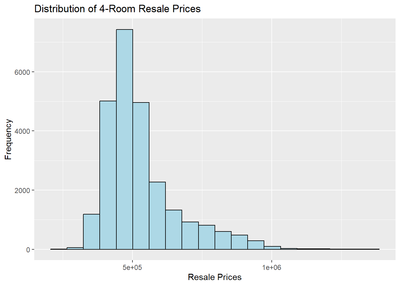
Note
From the histogram, we can see that it is skewed towards the right. This means that the transacted price were at a relative lower price.
resale_main_sf <- resale_main_sf %>%
mutate(`LOG_SELLING_PRICE` = log(PRICE))ggplot(data=resale_main_sf, aes(x=`LOG_SELLING_PRICE`)) +
geom_histogram(bins=20, color="black", fill="light blue")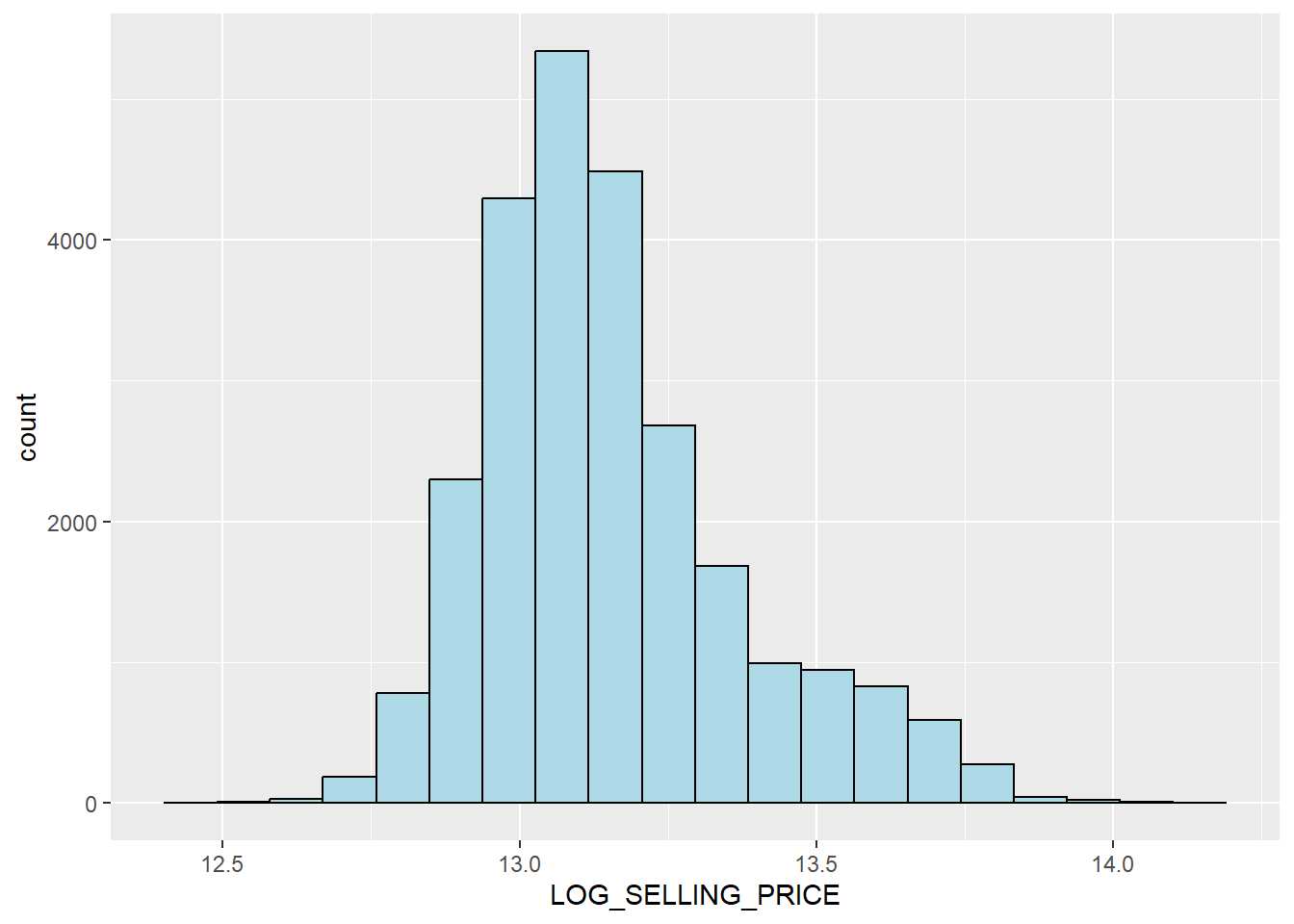
Note
We can see that after we log the values, it becomes slightly less skewed.
4.1.2 Viewing other category
AREA_SQM <- ggplot(data = resale_main_sf, aes(x = `AREA_SQM`)) +
geom_histogram(bins = 20, color = "black", fill = "light blue")
LEASE_MTHS <- ggplot(data = resale_main_sf, aes(x = `LEASE_MTHS`)) +
geom_histogram(bins = 20, color = "black", fill = "light blue")
PROX_CBD <- ggplot(data = resale_main_sf, aes(x = `PROX_CBD`)) +
geom_histogram(bins = 20, color = "black", fill = "light blue")
PROX_BUS <- ggplot(data = resale_main_sf, aes(x = `PROX_BUS`)) +
geom_histogram(bins = 20, color = "black", fill = "light blue")
PROX_CHILDCARE <- ggplot(data = resale_main_sf, aes(x = `PROX_CHILDCARE`)) +
geom_histogram(bins = 20, color = "black", fill = "light blue")
PROX_ELDERCARE <- ggplot(data = resale_main_sf, aes(x = `PROX_ELDERCARE`)) +
geom_histogram(bins = 20, color = "black", fill = "light blue")
PROX_HAWKER <- ggplot(data = resale_main_sf, aes(x = `PROX_HAWKER`)) +
geom_histogram(bins = 20, color = "black", fill = "light blue")
PROX_GOODPRIMARY <- ggplot(data = resale_main_sf, aes(x = `PROX_GOODPRIMARY`)) +
geom_histogram(bins = 20, color = "black", fill = "light blue")
PROX_PARK <- ggplot(data = resale_main_sf, aes(x = `PROX_PARK`)) +
geom_histogram(bins = 20, color = "black", fill = "light blue")
PROX_SUPERMARKET <- ggplot(data = resale_main_sf, aes(x = `PROX_SUPERMARKET`)) +
geom_histogram(bins = 20, color = "black", fill = "light blue")
PROX_SHOPPING <- ggplot(data = resale_main_sf, aes(x = `PROX_SHOPPING`)) +
geom_histogram(bins = 20, color = "black", fill = "light blue")
PROX_MRT <- ggplot(data = resale_main_sf, aes(x = `PROX_MRT`)) +
geom_histogram(bins = 20, color = "black", fill = "light blue")
WITHIN_350M_KINDERGARTEN <- ggplot(data = resale_main_sf, aes(x = `WITHIN_350M_KINDERGARTEN`)) +
geom_histogram(bins = 20, color = "black", fill = "light blue")
WITHIN_350M_CHILDCARE <- ggplot(data = resale_main_sf, aes(x = `WITHIN_350M_CHILDCARE`)) +
geom_histogram(bins = 20, color = "black", fill = "light blue")
WITHIN_350M_BUS <- ggplot(data = resale_main_sf, aes(x = `WITHIN_350M_BUS`)) +
geom_histogram(bins = 20, color = "black", fill = "light blue")
WITHIN_1KM_PRIMARY <- ggplot(data = resale_main_sf, aes(x = `WITHIN_1KM_PRIMARY`)) +
geom_histogram(bins = 20, color = "black", fill = "light blue")
ggarrange(AREA_SQM, LEASE_MTHS, PROX_CBD, PROX_BUS, PROX_CHILDCARE, PROX_ELDERCARE, PROX_HAWKER, PROX_GOODPRIMARY, PROX_PARK, PROX_SUPERMARKET, PROX_SHOPPING, PROX_MRT, WITHIN_350M_KINDERGARTEN, WITHIN_350M_CHILDCARE, WITHIN_350M_BUS, WITHIN_1KM_PRIMARY, ncol = 3, nrow = 6)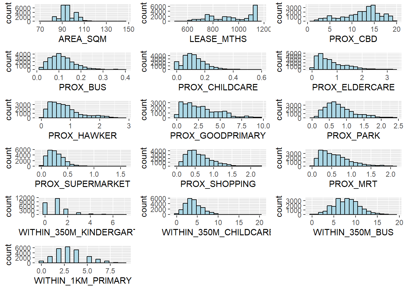
4.1.3 Viewing the Distribution using Boxplot
ggplot(data = resale_main_sf, aes(x = '', y = PRICE)) +
geom_boxplot() +
labs(x = '', y = 'Resale Prices')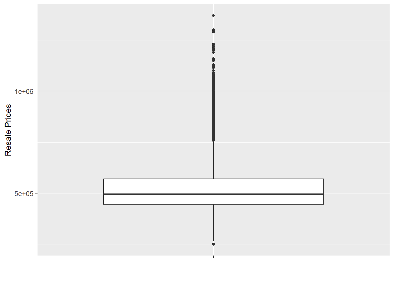
summary(resale_main_sf$PRICE) Min. 1st Qu. Median Mean 3rd Qu. Max.
250000 445000 495000 529142 570000 1370000
Note
We can see that there are quite a few outliers like the min and max selling at extremes. But mainly the price ranges from 554k to 570k
4.1.4 Point Map
tmap_mode("view")
tmap_options(check.and.fix = TRUE)
tm_shape(resale_main_sf)+
tm_dots(col = "PRICE",
alpha = 0.6,
style = "quantile",
popup.vars=c("block"="block", "street_name"="street_name", "flat_model" = "flat_model", "town" = "town", "PRICE" = "PRICE", "LEASE_MTHS", "LEASE_MTHS")) +
tm_view(set.zoom.limits = c(11, 14))